Guest post by Noel Salmeron, 2023 Senior Data Science Fellow for the Industry Documents Library and Data Science Initiative.

Hi everyone! I had the opportunity of interning for the Industry Documents Library in coordination with the Data Science Initiative as the Senior Data Science Fellow for the Summer of 2023. I am working towards my Bachelor’s degree in Data Science and minoring in Education, and I plan to graduate in May 2024. I feel grateful that I could earn this position with UCSF and work with the fascinating Industry Documents Library as I realize how valuable archives and data are, especially when doing my own research. The Data Science Initiative was extremely helpful in teaching me Machine Learning and Natural Language Processing topics pertinent to the project and valuable for my future in data science.

Project Background

Currently, the Industry Documents Library contains more than 18 million documents relating to public health, as well as thousands of audiovisual materials, such as “recordings of internal focus groups and corporate meetings, depositions of tobacco industry employees, Congressional hearings, and radio and TV cigarette advertisements.” With this project, we wanted to evaluate the transcription accuracy of digital archives and its impact on documentation and the creation of subject words and descriptions for such archives.

Project Team

• Kate Tasker, Industry Documents Library Managing Archivist
• Rebecca Tang, Industry Documents Library Applications Programmer (and Junior Fellows Advisor)
• Geoffrey Boushey, Head of Data Engineering (and Senior Fellow Advisor)
• Rachel Taketa, Industry Documents Library Processing and Reference Archivist
• Melissa Ignacio, Industry Documents Library Program Coordinator
• Noel Salmeron, Senior Data Science Fellow
• Adam Silva, Junior Data Science Fellow
• Bryce Quintos, Junior Data Science Fellow

Project Terminology

Here are a few important terms to note!

• Metadata: a set of data that describes other data (i.e., author, date published, file size, etc.)
• Classification: categorizing objects (or text) into organized groups
• Text cleaning: reducing complex text to simple text for more efficient use in Natural Language Processing

And a few terms were used interchangeably throughout this project!

• Description / Summary
  • A condensed version of some text
• Subject / Tag / Keyword / Topic
  • A single word that helps to define the text or frequently appears within the text

Project Objectives

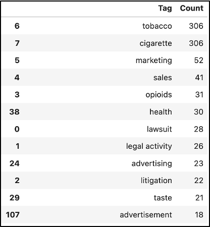
Overall, the project had a couple of main objectives. The team wanted to train a Machine Learning model to extract subjects from Industry Documents Library video transcripts and evaluate the accuracy of the machine-generated subjects. We planned to utilize the junior interns’ datasheet they created with subjects and descriptions for over 300 videos to train the model for each tag we chose to analyze.

(The video transcripts were generated beforehand by Google AutoML with the help of Geoffrey Boushey).

Transcript Cleaning

Once the video transcripts were created from Google AutoML, I was able to clean the text using techniques I learned from previous Data Science Initiative workshops. The “Machine Learning NLP Prep” workshop techniques were especially helpful for this portion of the project. I began by setting all 324 transcripts in our dataframe to a lowercase format. This helps simplify text analysis in the long run, especially when avoiding case sensitivity complications. My next step was to remove stop words, which are common and redundant words such as articles, conjunctions, and prepositions. This was possible with the Natural Language Toolkit library for Python, which contains a list of stop words I could add to since I especially noticed ‘p.m.’ and ‘a.m.’ appearing in depositions. I continued by removing everything that isn’t alphabetic using a regular expression (or regex), a sequence of characters corresponding to a pattern to be matched. Any single characters or two character pairs were also removed. Finally, it was essential to stem words to be able to group common words without worrying about suffixes.

ML Model Creation using ID and subject/tag

After text cleaning, we set video IDs as their indices in our running dataframe to efficiently and consistently identify them. Our running dataframe consisted of a row for each of the 324 videos with columns that denoted their ID, subject words, transcript, and a category value of  ‘0’ for ‘no’ or ‘1’ for ‘yes’ that corresponded to whether or not the video’s subjects words included the specific tag we were after in each single-tag analysis.

To provide a more concrete example, we will use the “lawsuit” tag, which means each video was denoted with a ‘1’ in the category column if it contained the “lawsuit” tag from the junior interns’ datasheet.

Continuing, we created training and test sets from the dataframe with a 50/50 split. This was followed by a pipeline of several operations in a sequence that included Count Vectorization and Random Forest Classification. Count Vectorization is a method in Natural Language Processing to convert text into numerical values primed for Machine Learning. This way, we can note word frequency in each word for each transcript. Furthermore, Random Forest Classification is a collection of decision trees that make binary decisions based on input and continually “bootstraps” (re-samples) from the training data set to make predictions about whether or not a video contained the “lawsuit” tag.

Features for Each Tag

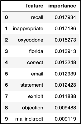
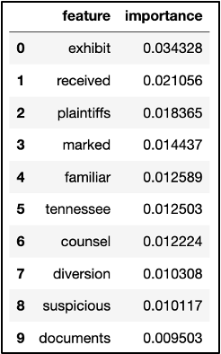
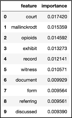
We then gathered feature words and their importance values as to how they supported the model in determining if a video belonged to the “lawsuit” tag. These feature words included “exhibit,” “plaintiffs,” “counsel,” and “documents,” which change every time we run the model. It appears the less common words also slipped through, such as the company name “Mallinckrodt,” which may not appear as important in other transcript datasets relating to lawsuits.

Cross Validation and Match Probability

Moving forward, we used Cross Validation to verify that the model’s performance was not drastically different with different training and test subsets from the running dataframe. Following this process, we were able to create a dataframe that included a column “y_adj” to indicate “Not” for the video not falling under the “lawsuit” tag and an indication of “Match” otherwise. Moreover, we included two columns, “prob_no_match” and “prob_match,” that denote the model’s assessment of the probability that a video doesn’t fit under “lawsuit” or does, respectively.

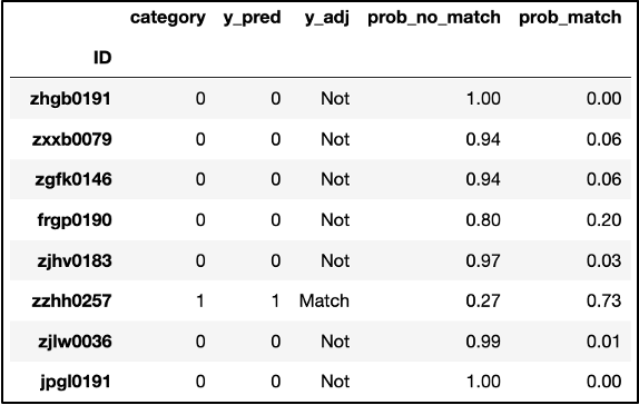
We also ran some code that narrowed down the dataframe to videos where the model incorrectly predicted a video’s match.

This is where we began to run into issues with this dataset since it contained a relatively small amount of videos and, therefore, a low number of videos where the “lawsuit” tag applied. The “lawsuit” tag was filed under only 26 of the 324 videos, a mere 8 percent of the dataset. It was also quite difficult to discern an appropriate threshold for whether or not a video transcript should be marked as a match to a tag because the videos that the model marked incorrectly usually appear to have significantly different probabilities for matching.

This caused our models for tags with counts under 25 or so to result in a non-existent F-score, as well as precision and recall, but a high accuracy which I will explain shortly. Meanwhile, an F-score is critical in providing an overall measure or metric for the performance of a Machine Learning model using its precision and recall.

Precision & Recall

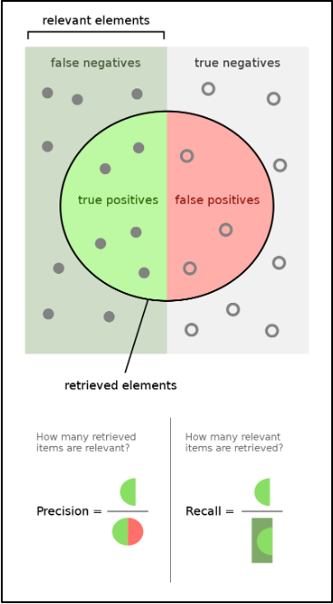
Diving into Precision and Recall, Precision can be defined as the proportion of correct positive predictions in the number of predicted positive values, while Recall is the proportion of correct positive predictions in the number of actual positive values.

In this project, the positive values would be video matches for a tag, so in terms of the project, precision is the proportion of correct match predictions out of the predicted matches, and recall is the proportion of correct match predictions out of the actual, true matches. In addition, Accuracy refers to the comprehensive correctness of all positive and negative predictions.

This image may also help visualize the precision/recall relationship:

Thresholds

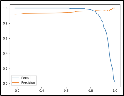
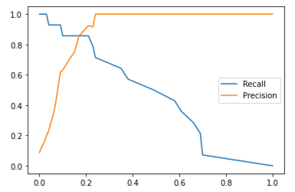
Another step we took in this project’s analysis was creating precision-recall curves for specified thresholds by the Scikit-learn library that allows for Machine Learning in Python. This way, we could recognize that as the threshold for the probability of a match increases, the precision slowly increases from about 90 percent to 100 percent. In comparison, the recall decreases from 100 percent to 0 percent.

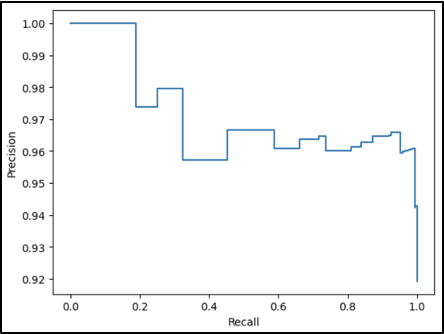
This can be explained by referring back to the definitions of precision and recall! Suppose the threshold for the probability of a match increases and becomes stricter. In that case, precision (the proportion of correct matches out of predicted matches) will only increase as the requirement for a video to be labeled as a match becomes stricter. Regarding the recall (the proportion of correct match predictions out of the actual matches), it becomes clear that since there is more precision, there will be no videos incorrectly marked as matches or any videos correctly marked as matches.

Opportunities for Further Research

There were a few concerns and curiosities that I ended the beginning of this project with since it was simply a pilot, and there is much more to be explored. This includes more text cleaning in subjects/tags and transcripts to make the Natural Language Processing as streamlined as possible. Additionally, it would be crucial to explore this same analysis of subjects/tags for descriptions/summaries that we could not get to. Having a fully-developed human-made datasheet for a larger dataset to explore would also be incredibly useful.

Conclusion

I am pleased to have been a part of this team with UCSF’s Industry Documents Library and Data Science Initiative this summer, as it provided me with extensive real-world experience in data analysis, machine learning, and natural language processing. It truly puts into perspective how much valuable data is out there and all of the fascinating analysis you can conduct.

Prior to this summer, I had worked with various datasets in classes, but I felt inspired by the IDL’s endeavor to enhance its vast collection and make it easier for users to search through documents with supplementary metadata. I can especially appreciate this as I have spent countless hours sifting through documents for research papers in the past. Once the subject and description generations are in full effect, I can only imagine the potential of this data and what it could lead to, as I hope it supports other people’s work.

I also tremendously appreciate the time and effort the junior interns, Adam and Bryce, put into populating their datasheet after watching hundreds of videos. Their work was foundational to getting this project running.

I also want to express my appreciation for Geoffrey and Rebecca throughout this summer for working closely with me, making me feel welcome, and addressing any concerns or questions I had during my fellowship. I am incredibly grateful for this work experience with exceptional communication, collaboration, and kindness.

Thank you to UCSF and everyone on this team for an enjoyable and fascinating fellowship experience!

---

Addendum: When Should We Apply a Subject Tag to an Uncategorized Document?

By Geoff Boushey, UCSF Library Head of Data Engineering

Overview

Noel described the process for creating a machine learning (ML) model, analyzing the features that go into classifying a document, and applying the model to estimate the probability that a transcript generated from the Tobacco or Opioid collection should be included in a subject tag, such as “marketing,” “legal,” or “health.”

Because most tags in the collection show up in less than 10% of the records in our training and testing set, we shouldn’t expect most tags to apply to most records. As a result, we’re looking for a relatively rare event. If we were only concerned with the overall accuracy or our model, we could achieve 90% effectiveness by never applying a specific tag to a record.

The output from our machine learning model reflects this low probability. By default, our machine learning model would only include a tag if it estimates that the probability of a match exceeds 50%. Because we’re trying to predict a relatively rare event (again, a specific tag would only apply to at most 10% of the records in a collection), it’s unlikely that we’ll have many predictions that exceed this threshold. In fact, when we test our model, we can see that records that clearly (based on human observation) belong to a specific category may have no more than a 30-40% estimated probability of belonging to this category according to the ML model. While this is below the default 50% threshold, it does represent a much higher probability than random chance, (30-40% vs 10%).

We don’t want to erroneously include a tag too often, or it will become clutter. We don’t want to erroneously exclude it too often, or researchers will miss out on relevant record matches. We may want to lower the threshold for determining when to apply a tag to a particular record, but the right threshold isn’t always clear, and can vary depending on the frequency of a tag, the accuracy of our model, and the scenario-dependent benefit or harm of false positives versus false negatives.

The harm of false positives or negatives depends heavily on the research or use scenario. For example, a researcher who wants to retrieve all reasonably likely matches and is not concerned with the inclusion of a few documents that are not related to litigation might want to set the threshold very low, even below 10%. Alternatively, a researcher might simply wish to sample a small number of litigation-related documents with a very high level of accuracy. In this case, a high threshold would be more beneficial.

Precision and Recall curves can help find an optimal threshold that strikes the right balance between false positives and false negatives.

Technical Considerations and Limitations

Because our initial dataset is small (only 300 human reviewed records are available for supervised classification), and many of the tags only show up in 10% of the records, we limit our initial analysis to a small set of metadata tags. Because these tags are human-generated and do not conform to a limited and controlled vocabulary, there is inconsistency in the training data as well. Some tags are redundant, showing up in clusters (legal and litigation, for instance, have a 95%+ overlap). Other times, two categories that might be better approached as a single category cause a split that may greatly reduce the effectiveness of an ML based classifier. Human ambiguity is often amplified when used to train ML models, and we see that effect at work here.

Precision-Recall Curves

Because there is a class imbalance between positive and negative categorization (including versus excluding a tag) and false positives are unlikely to be a serious problem (though, as discussed above, there may be some scenarios, such as sampling, where we would want to avoid them), we’ll take a look at precision-recall curves for a few of the more commonly occurring tags.

For quick reference, *Precision* refers to how often a positive classification was correct. For example, if our model predicted that a “Legal” tag should apply correctly 9 times and incorrectly 1 time, the Precision would be 90%. *Recall* refers to how often a positive classification was accurately detected. For example, if 10 records should have been classified as Legal, and our model detected 8 of them, our recall rate would be 80%. Ideally, we would like to strike some kind of balance between these two metrics, something we can achieve by raising or lowering the probability threshold for including a record in a tag. For example, if our model assigned a 30% chance that a particular record should be classified as “Legal”, we might or might not set that assignment based on whether we are trying to improve precision or recall.

For a more technical/mathematical discussion of Precision and Recall, please consult the scikit learn documentation at:

https://scikit-learn.org/stable/auto_examples/model_selection/plot_precision_recall.html

Workbook

The jupyter notebook implementing a Precision-Recall visualization for the “Legal” tag is

available at:

https://github.com/geoffswc/IDL-DSOS-2023/blob/main/Precision-Recall-Tag.ipynb

This workbook uses the scikit-plot module from scikit-learn to generate a precison-recall curve for a tag used in the classification model. Keep in mind that there isn’t much benefit to analyzing tags that show up in less than 10% of the records, and some tags may result in an error, as positive observations may be so rare (fewer than 1-2% of the records) that there is insufficient data to train or apply an ML model (a random test/train split may have *no* observations for a rare tag such a small dataset).

The visualizations generated by this workbook are available in the next section.

Visualization and Interpretation

This section displays the PR curve for “Legal”, a tag that shows up in approximately 10% of the training records. Keep in mind that common tags like “Tobacco”, which show up in 90% of the records, are auto-assigned based on the source of the collection, and do not represent the common use case. As a result, “Legal” will provide a better overview for a common tag that does not apply to most records, and performs relatively well in our predictive model.

Precision-Recall

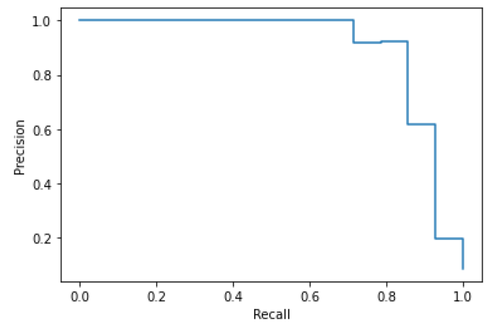
The precision recall curve for Legal indicates a wide threshold range that preserves usable precision and recall levels. Very high or low thresholds cause degradation of model performance, but precision and recall above 80% are available with flexibility to optimize for one or the other.

Precision/Recall-Threshold

This chart plots both precision and recall curves on the Y axis with the threshold level on the X axis. We see a rapid improvement of precision with a gradual, near-linear decrease in recall, indicating an effective threshold range well below 50%.

Production Application

Although our current data set is small, these results suggest that there is some value in using a supervised classification model to extend metadata to uncategorized documents based on ML generated transcript, though there are a number of challenges, and integrating these techniques into production would involve a number of decisions that are outside the scope of this pilot.

Challenges

A production rollout of an ML based model similar to this pilot would likely run into a number of issues with scale, such as:

• Training Data: our supervised machine learning model requires a set of categorized transcripts for training. This is a very time and labor intensive undertaking. We may not be able to create a sufficiently large and broad training dataset to create a meaningful model that covers even the most common tags.

• Varying Thresholds: The ideal threshold will vary based on the model performance for each individual tag and the research objectives. This variance, combined with the scale of processing required, may make customizable searches based on tag probability unrealistic in a production system.

• Availability of Transcripts: The tobacco, opioid, and other industry documents collections contain a large number of files (current estimate is 18 million), many are video or audio files without transcriptions. Without transcriptions available, it won’t be possible to apply the results of an ML model to make predictions for uncategorized documents.

Recommendations

This pilot does provide a template for an interesting and promising approach, and researchers may be interested in building their own ML models to analyze the transcripts in the collections.

We could provide some of this utility without a full production integration through the following:

• Pre-Built Transcription Datasets: The Industry Documents Library website currently provides pre-built transcription datasets for many image record collections. A similar initiative to provide transcriptions for video and audio would provide substantial benefit for researchers, independent of the ML based classification model.

• Classification Probability Estimates: Instead of integrating classification probabilities or tags into search, we could provide the ML output for each record in a pre-built dataset. This would leave the decision for setting a threshold up to researchers, but it would avoid the need to re-generate results based on model performance and researcher scenario for each tag. This approach might allow researchers to benefit from partial information.

• Generalized ML Models: Several AI tools, such as Google AutoML AI, do provide pre-trained models that can provide categorization. Because these models wouldn’t be trained specifically on our metadata, they may not capture the kind of classification most relevant to researchers, but they would eliminate the need for the very labor intensive generation of a training data set.

The UCSF Industry Documents Library (IDL) and Data Science Initiative (DSI) teams are excited to be working with three Data Science Fellows this summer. The Data Science Fellows are part of a joint IDL-DSI project to explore machine learning technologies to create and enhance descriptive metadata for thousands of audio and video recordings in IDL’s archival collections.  This year’s summer program includes two junior fellows and one senior fellow.

Our junior fellows are tasked with manually assigning or improving metadata fields such as title, description, subject, and runtime for a selection of videos in IDL’s collection on the Internet Archive. This is a detailed and time-consuming task, which would be costly to perform for the entire collection. In contrast, our senior fellow is using transcriptions of the videos, which we have generated with Google’s AutoML tool, to explore different technologies to automatically extract the descriptive information. We’ll then compare the human-generated data with the machine-generated data to assess accuracy.  The hope is that IDL can develop a workflow for using machine learning to create or improve metadata for many other videos in our collections.

Our Junior Data Science Fellows are Bryce Quintos and Adam Silva. Bryce and Adam are both participating in the San Francisco Unified School District (SFUSD) Career Pathway Summer Fellowship Program. This six-week program provides opportunities for high school students to gain work experience in a variety of industries and to expand their learning and skills outside of the classroom. Bryce and Adam are learning about programming and creating transcription for selected audiovisual materials. The IDL thanks SFUSD and its partners for running this program and providing sponsorship support for our fellows.

Noel Salmeron is our Senior Data Science Fellow participating in Life Science Cares Bay Area’s Project Onramp. Noel is using automated transcription tools to extract text from audiovisual files, run sentiment and topic analyses, and compare automated results to human transcription. Noel also provides guidance and mentoring to the Junior Fellows.

Our Fellows have shared a bit about themselves below. Please join us in recognizing Bryce, Adam, and Noel for their contributions to the UCSF Library this summer!

Hi everyone! My name is Bryce Quintos and I am an incoming freshman at Boston University. I
hope to major in biochemistry and work in the biotechnology and pharmaceutical field. As someone who is interested in medical research and science, I am incredibly honored for the opportunity to help organize the Industry Documents Library at UCSF this summer and learn more about computer programming. I can’t wait to meet all of you!

Hi, my name is Adam Silva and I am a Junior Intern for the UCSF Library. Currently, I am 17 years old and I am going into my senior year at Abraham Lincoln High School in San Francisco. I am part of Lincoln High School’s Dragon Boat team and I am also a part of Boy Scout Troop 15 in San Francisco. My favorite activities include cooking, camping, hiking, and backpacking. My favorite thing that I did in Boy Scouts was backpacking through Rae Lakes for a week. I am excited to work as a Junior Intern this year because working online rather than in person is new to me. I look forward to working with other employees and gaining the experience of working in a group.

My name is Noel Salmeron and I am a third-year data science major and education minor at UC Berkeley. I’m excited to work with everyone this summer and looking forward to contributing to the Industry Documents Library!

The 18th International Conference on Digital Preservation (iPRES) took place from September 12-16, 2022, in Glasgow, Scotland. First convened in 2004 in Beijing, iPRES has been held on four different continents and aims to embrace “a variety of topics in digital preservation – from strategy to implementation, and from international and regional initiatives to small organisations.” Key values are inclusive dialogue and cooperative goals, which were very much centered in Glasgow thanks to the goodwill of the attendees, the conference code of conduct, and the significant efforts of the remarkable Digital Preservation Coalition (DPC), the iPRES 2022 organizational host.

I attended the conference in my role as the UCSF Industry Documents Library’s managing archivist to gain a better understanding of how other institutions are managing and preserving their rapidly-growing digital collections. For me and for many of the delegates, iPRES 2022 was the first opportunity since the COVID pandemic began to join an in-person conference for professional conversation and exchange. It will come as no surprise to say that gathering together was incredibly valuable and enjoyable (in no small part thanks to the traditional Scottish ceilidh dance which took place at the conference dinner!) The Program Committee also did a fantastic job designing an inclusive online experience for virtual attendees, with livestreamed talks, online social events, and collaborative session notes.

Session themes focused on Community, Environment, Innovation, Resilience, and Exchange. Keynotes were delivered by Amina Shah, the National Librarian of Scotland; Tamar Evangelestia-Dougherty, the inaugural director of the Smithsonian Libraries and Archives; and Steven Gonzalez Monserrate, an ethnographer of data centers and PhD Candidate in the History, Anthropology, Science, Technology & Society (HASTS) program at the Massachusetts Institute of Technology.

Every session I attended was excellent, informative, and thought-provoking. To highlight just a few:

Amina Shah’s keynote “Video Killed the Radio Star: Preserving a Nation’s Memory” (featuring the official 1980 music video by the Buggles!) focused on keeping up with the pace of change at the National Library of Scotland by engaging with new formats, new audiences, and new uses for collections. She noted that “expressing value in a key part of resilience” and that the cultural heritage community needs to talk about “why we’re doing digital preservation, not just how.” This was underscored by her description of our world as a place where the truth is under attack, that capturing the truth and finding a way to present it is crucial, and that it is also crucial that this work be done by people who aren’t trying to make a profit from it.

“Green Goes with Anything: Decreasing Environmental Impact of Digital Libraries at Virginia Tech,” a long paper presented by Alex Kinnaman as part of the wholly excellent Environment 1 session, examined existing digital library practices at Virginia Tech University Libraries, and explored changes in documentation and practice that will foster a more environmentally sustainable collections platform. These changes include choosing the least-energy consumptive hash algorithms (MD4 and MD5) for file fixity checks; choosing cloud storage providers based on their environmental practices; including environmental impact of a digital collection as part of appraisal criteria; and several other practical and actionable recommendations.

The Innovation 2 session included two short papers (by Pierre-yves Burgi, and by Euan Cochrane) and a fascinatingly futuristic panel discussion posing the question “Will DNA Form the Fabric of our Digital Preservation Storage?” (Also special mention to the Resilience 1 session which presented proposed solutions for preserving records of nuclear decommissioning and nuclear waste storage for the very long term – 10,000 years!)

Tamar Evangelestia-Dougherty’s keynote Digital Ties That Bind: Effectively Engaging With Communities For Equitable Digital Preservation Ecosystems was an electric presentation that called unequivocally for centering equity and inclusion within our digital ecosystems, and for recognizing, respecting, and making space for the knowledge and contributions of community archivists. She called out common missteps in digital preservation outreach to communities, and challenged all those listening to “get more people in the room” to include non-white, non-Western perspectives.

“’…provide a lasting legacy for Glasgow and the nation’: Two years of transferring Scottish Cabinet records to National Records of Scotland,” a short paper by Garth Stewart in the Innovation 4 session, touched on a number of challenges very familiar to the UCSF Industry Documents Library team! These included the transfer of a huge volume of recent and potentially sensitive digital documents, in redacted and unredacted form; a need to provide online access as quickly as possible; serving the needs of two major access audiences – the press, and the public; normalizing files to PDF in order to present them online; and dealing with incomplete or missing files.

And so much more, summarized by the final keynote speaker Steven Gonzalez Monserrate after his fantastical storytelling closing talk on the ecological impact of massive terrestrial data centers and what might come after “The Cloud” (underwater data centers? Clay tablets? Living DNA storage?). And, I didn’t even mention the Digital Preservation Bake Off Challenge…

After the conference I also had the opportunity to visit the Archives of the Royal College of Physicians and Surgeons of Glasgow, where our tour group was welcomed by the expert library staff and shown several fascinating items from their collections, including an 18th century Book of Herbal Remedies (which has been digitized for online access).

After five collaborative and collegial days in Glasgow, I’m looking forward to bringing these ideas back to our work with digital archival collections here at UCSF. Many thanks to iPRES, the DPC, the Program Committee, the speakers and presenters, and all the delegates for building this wonderful community for digital preservation!

This is a guest post from Lubov McKone, the Industry Documents Library’s 2022 Data Science Senior Fellow.

This summer, I served as the Industry Documents Library’s Senior Data Science Fellow. A bit about me – I’m currently pursuing my MLIS at Pratt Institute with a focus in research and data, and I’m hoping to work in library data services after I graduate. I was drawn to this opportunity because I wanted to learn how libraries are using data-related techniques and technologies in practice – and specifically, how they are contextualizing these for researchers.

Project Background

The UCSF Industry Documents Library is a vast collection of resources encompassing documents, images, videos, and recordings. These materials can be studied individually, but increasingly, researchers are interested in examining trends across whole collections, or subsets of it. In this way, the Industry Documents Library is also a trove of data that can be used to uncover trends and patterns in the history of industries impacting public health. In this project, the Industry Documents Library wanted to investigate what information is lost or changed when its collections are transformed into data. 

There are many ways to generate data from digital collections. In this project we focused on a combination of collections metadata and computer-generated transcripts of video files. Like all information, data is not objective but constructed. Metadata is usually entered manually and is subject to human error. Video transcripts generated by computer programs are never 100% accurate. If accuracy varies based on factors such as the age of the video or the type of event being recorded, how might this impact conclusions drawn by researchers who are treating all video transcriptions as equally accurate? What guidance can the library provide to prevent researchers from drawing inaccurate conclusions from computer-generated text?

Project Summary

Research Questions

Based on the background and the goals of the Industry Documents Library, the project team identified the following research questions to guide the project:

• Taking into account factors such as year and runtime, how does computer transcription accuracy differ between television commercials and court proceedings?
• How might transcription accuracy impact the conclusions drawn from the data? 
• What guidance can we give to researchers to prevent uninformed conclusions?

Uses

This project is a case study that evaluates the accuracy of computer-generated transcripts for videos within the Industry Documents Library’s Tobacco Collection. These findings provide a foundation for UCSF’s Industry Documents Library to create guidelines for researchers using video transcripts for text analysis. This case study also acts as a roadmap and a collection of instructional materials for similar studies to be conducted on other collections. These materials have been gathered in a public github repo, viewable here. 

Sourcing the Right Data

At the beginning of the project, we worked with the Junior Fellows to determine the scope of the project. The tobacco video collection contains 5,249 videos that encompass interviews, commercials, court proceedings, press conferences, news broadcasts, and more. We wanted to narrow our scope to two categories that would illustrate potential disparities in transcript accuracy and meaning. After transcribing several videos by hand, the fellows proposed commercials and court proceedings as two categories that would suit our analysis. We felt 40 would be a reasonable sample size of videos to study, so each fellow selected 10 videos from each category, selecting videos with a range of years, quality, and runtimes. The fellows were selecting videos from a list that was generated by the InternetArchive python API, containing video links and metadata such as year and runtime.

Computer & Human Transcripts

Once the 40 videos were selected, we extracted transcripts from each URL using the Google AutoML API for transcription. We saved a copy of each computer transcription to use for the analysis, and provided another copy to the Junior Fellows, who edited them to accurately reflect the audio in the videos. We saved these copies as well for comparison to the computer-generated transcription.

Comparing Transcripts

To compare the computer and human transcripts, we conducted research on common metrics for transcript comparison. We came up with two broad categories to compare – accuracy and meaning. 

To compare accuracy, we used the following metrics:

• Word Error Rate – a measure of how many insertions, deletions, and substitutions are needed to convert the computer-generated transcript into the reference transcript. We subtracted this number from 1 to get the Word Accuracy Rate (WAR).
• BLEU score – a more advanced algorithm measuring n-gram matches between the transcripts, normalized for n-gram frequency.
• Human-evaluated accuracy –  a score from Poor, Fair, Good, and Excellent assigned by the fellows as they were editing the computer-generated transcripts.
• Google AutoML confidence score –  a score generated by Google AutoML during transcript generation indicating how accurate Google believes its transcription to be.

To compare meaning, we used the following metrics:

• Sentiment – We generated sentiment scores and magnitude for both sets of transcripts. We wanted to see whether the computer transcripts were under- or over- estimating sentiment, and whether this differed across categories. 
• Topic modeling – We ran a k-means topic model for two categories to see how closely the computer transcripts matched the pre-determined categories vs. how closely they were matched by the human transcripts

Findings & Recommendations

Relationships in the data

From an initial review of the significant correlations in the data, we gained some interesting insights. As shown in the correlation matrix, AutoML confidence score, fellow accuracy rating, and Word Accuracy Rate (WAR) are all significantly positively correlated. This means that the AutoML confidence score is a relatively good proxy for transcript accuracy. We recommend that researchers who are seeking to use computer-generated transcripts look to the AutoML confidence score to get a sense of the reliability of the computer-generated text they are working with.

We also found a significant positive correlation between year and fellow accuracy rating, Word Accuracy Rate, and AutoML confidence score – suggesting that the more recent the video, the better the quality. We suggest informing researchers that newer videos may generate more accurate computer transcriptions.

Transcript accuracy over time

One of the Junior Fellows suggested that we look into whether there is a specific cutoff year where transcripts become more accurate. As shown in the visual below, there’s a general improvement in transcription quality after the 1960s, but not a dramatic one. Interestingly, this trend disappears when looking at each video type separately.

Transcript accuracy by video type

When comparing transcript accuracy between the two categories, we found that our expectations were challenged. We expected the accuracy of the advertising video transcripts to be higher, because advertisements generally have a higher production quality, and are less likely to have features like multiple people speaking over each other that could hinder transcription accuracy. However, we found that across most metrics, the court proceeding transcripts were more accurate. One potential reason for this is that commercials typically include some form of singing or more stylized speaking, which Google AutoML had trouble transcribing. We recommend informing researchers that video transcripts from media that contain singing or stylized speaking may be less accurate.

The one metric that the commercials were more accurate in was BLEU score, but this should be interpreted with caution. BLEU score is supposed to range from 0-1, but in our dataset its range was 0.0001 – 0.007. BLEU score is meant to be used on a corpus that is broken into sentences, because it works by aggregating n-gram accuracy on a sentence level, and then averaging the sentence-level accuracies across the corpus. However, the transcripts generated by Google AutoML did not contain any punctuation, so we were essentially calculating BLEU score on a corpus-length sentence for each transcript. This resulted in extremely small BLEU scores that may not be accurate or interpretable. For this reason, we don’t recommend the use of the BLEU score metric on transcripts generated by Google AutoML, or on other computer-generated transcripts that lack punctuation.

Transcript sentiment

We looked to sentiment scores to evaluate differences in meaning between the test and reference transcripts. As we expected, commercials, which are sponsored by the companies profiting off of the tobacco industry, tend to have a positive sentiment, while court proceedings, which tend to be brought against these companies, tend to have a negative sentiment. As shown in the plot to the left, the sentiment of the computer transcripts was a slight underestimation in both video types, though this was not too dramatic of an underestimation. 

Opportunities for Further Research

Throughout this project, it was important to me to document my work and generate a research dataset that could be used by others interested in extended this work beyond my fellowship. There were many questions that we didn’t get a chance to investigate over the course of this summer, but my hope is that the work can be built upon – maybe even by a future fellow! This dataset lives in the project’s github repository under data/final_dataset.csv.

One aspect of the data that we did not investigate as much as we had hoped was topic modeling. This will likely be an important next step in assessing whether transcript meaning varies between the test and reference transcripts.

Professional Learnings & Insights

My main area of interest in the field of library data services is critical data literacy – how we as librarians can use conversations around data to build relationships and educate researchers about how data-related tools and technologies are not objective, but subject to the same pitfalls and biases as other research methods. Through my work as the Industry Documents Library Senior Data Science Fellow, I had the opportunity to work with a thoughtful team who is thinking ahead about how to responsibly guide researchers in the use of data. 

Before this fellowship, I wasn’t sure exactly how opportunities to educate researchers around data would come up in a real library setting. Because I previously worked for the government, I tended to imagine researchers sourcing data from government open data portals such as NYCOpenData, or other public data sources. This fellowship opened my eyes to how often researchers might be using library collections themselves as data, and to the unique challenges and opportunities that can arise when contextualizing this “internal” data for researchers. As the collecting institution, you might have more information about why data is structured the way it is – for instance, the Industry Documents Library created the taxonomy for the archive’s “Topic” field. However, you are also often relying on hosting systems that you don’t have full control over. In the case of this project, there were several quirks of the Internet Archive API that made data analysis more complicated – for example, the video names and identifiers don’t always match. I can see how researchers might be confused about what the library does and does not have control over.

Another great aspect of this fellowship was the opportunity to work with our high school Junior Fellows, who were both exceptional to work with. Not only did they contribute the foundational work of editing our computer-generated transcripts – tedious and detail-oriented work – they also had really fresh insights about what we should analyze and what we should consider about the data. It was a highlight to support them and learn from them.

I also appreciated the opportunity to work with this very unique and important collection. Seeing the breadth of what is contained in the Industry Documents Library opened my eyes to not only the wealth of government information that exists outside of government entities, but also to the range of private sector information that ought to be accessible to the public. It’s amazing that an archive like the Industry Documents Library is also so invested in thinking critically about the technical tools that it’s reliant upon, but I guess it’s not such a surprise! Thanks to the whole team and to UCSF for a great summer fellowship experience!

The Industry Documents Library (IDL) is excited to welcome three Data Science Fellows to our team this summer. The Data Science Fellows will be working with the IDL and with the UCSF Library Data Science Initiative (DSI) to to assess the impact of transcription accuracy on text analysis of digital archives, using the IDL collections.

Through tagging, human transcription, and computer-generated transcription, the team will assess how accuracy may differ between media or document types, and how and whether this difference is more or less pronounced in certain categories of media (for example, video recordings of focus groups, community meetings, court proceedings, or TV commercials, all of which are present in the IDL’s video collections). After identifying transcript accuracy in different media types, we aim to provide guidelines to researchers and technical staff for proper analysis, measurement, and reporting of transcript accuracy when working with digital media.

Our Junior Data Science Fellows are Rogelio Murillo and Lianne De Leon. Rogelio and Lianne are both participating in the San Francisco Unified School District (SFUSD) Career Pathway Summer Fellowship Program. This six-week program provides opportunities for high school students to gain work experience in a variety of industries and to expand their learning and skills outside of the classroom. Lianne and Rogelio will be learning about programming and creating transcription for selected audiovisual materials. The IDL thanks SFUSD and its partners for running this program and providing sponsorship support for our fellows.

Lubov McKone is our Senior Data Science Fellow and will be using automated transcription tools to extract text from audiovisual files, run sentiment and topic analyses, and compare automated results to human transcription. Lubov will also provide guidance and mentoring to the Junior Fellows.

Our Fellows have introduced themselves below. Please join us in welcoming Rogelio, Lianne, and Lubov to the UCSF Library this summer!

Hi my name is Lianne R. de Leon and I go to Phillip and Sala Burton High School as a rising senior. I love playing volleyball in my free time and you may see me at numerous open gyms around the city. In the future I hope to major in computer science or computer engineering. I’m looking forward to meeting many wonderful people here at UCSF and learning more about the data science industry from the inside.

Hi, my name is Rogelio Murillo and I’m a rising junior at Ruth Asawa School of the Arts. I enjoy playing a variety of music and percussion. I’ve played Japanese Taiko, Afro Brazilian drumming, and Latin Jazz. I’m also learning guitar over the summer. I’m a responsible and respectful person.

My name is Lubov McKone and I’m currently pursuing my Masters in Library and Information Science from Pratt Institute in Brooklyn, NY. I also hold a Bachelor’s degree in Statistics, and prior to entering graduate school I worked as a data analyst in local government. My professional interests include supporting researchers in the accurate and responsible use of data, and I aspire to work as a data librarian in an academic library after graduation. Outside of work, I spend my time cooking, doing yoga, and writing music. I’m very excited to be joining the UCSF Industry Documents Library this summer, and I’m looking forward to learning more about how researchers use digital collections!

Please join us in giving a warm welcome to our two newest summer interns, May Yuan and Lianne de Leon!

May and Lianne are both participating in the San Francisco Unified School District (SFUSD) Career Pathway Summer Fellowship Program. This six-week program provides opportunities for high school students to gain work experience in a variety of industries and to expand their learning and skills outside of the classroom. Lianne and May will be working (remotely) with the UCSF Industry Documents Library (IDL), and we are grateful to SFUSD and its partners for sponsoring these internships.

May and Lianne will be working on several collection description projects with IDL this summer, including correcting and enhancing document metadata, and creating descriptions for audio-visual materials. They have provided their introductions below.

My name is May Yuan and I’m a junior at Raoul Wallenberg Traditional High School. During my free time, I enjoy reading, learning and trying new things, and helping others academically. I’m super excited to work here at the UCSF IDL to help provide valuable information to the public as well as learn more about the various documents, lawsuits, etc. myself; I also hope to enhance my productivity and organization skills during my time working here as these skills are crucial to college and everyday life in general. The career paths I’m interested in are bioengineering (bioinformatics/biostatistics), law, and finance.

Hi, my name is Lianne R. de Leon. I am a part of the Class of 2023 at Phillip and Sala Burton High School. In the past, I have worked on VEX EDR Robotics competition in 2018-2019. In my spare time I enjoy trying new foods and yoga. I aspire to become a computer hardware engineer and to travel across the entirety of Asia. I look forward to meeting and working with you all.

Please join us in giving a warm welcome to Khushi Bhat, who will be conducting a remote internship with the UCSF Industry Documents Library (IDL) this summer.

Khushi is currently a rising senior at Rutgers University where she is majoring in Biotechnology and minoring in Computer Science. This summer, she is working in the Industry Documents Library researching tools and methods to extract geographic locations from a collection of documents related to the tobacco industry’s influence in public policy.

Khushi will be conducting an independent course project to help the IDL team enhance descriptive metadata for our industry documents collections. We have long been aware of a research need to be able to filter documents by geographic location. Tobacco control researchers and other public health experts at UCSF and around the world use the documents in the Industry Documents Library to understand how corporations impact public health. This research is often used to inform policymakers who write laws and policies regulating the sale and use of products such as tobacco. Researchers and policymakers need information which relates to their local area such as their city, county, state, or country.

Geographic location is not currently included in IDL’s document-level metadata, and since IDL contains more than 15 million documents it is not feasible to manually catalog this information.

Khushi’s work will focus on researching Natural Language Processing (NLP) and Named Entity Recognition (NER) text analysis methods. She will investigate available tools which have the potential to automatically identify and label geographic information in text. Khushi’s research, recommendations, and pilot testing will help the IDL team outline workflows and strategies for enhancing our document metadata to include geographic information.

Khushi aspires to pursue a career in bioinformatics in the future and intends on pursuing higher education in this field upon graduation. In her spare time, Khushi enjoys dancing, baking, and hiking. Prior to joining Rutgers, she was an avid Taekwondo practitioner (and has a 2nd degree black belt to show for it!)

The Medical Heritage Library 10th Anniversary Conference took place on November 13, 2020. UCSF Archives and Special Collections staff attended the day of virtual presentations, and our Industry Documents Library archivists delivered a talk titled “Smoke on Screens: Audiovisual Evidence of the Tobacco Industry’s Harms to Public Health.”

The conference was convened to celebrate a decade of digitizing and making available medical history resources. Keynote speaker Dr. Jaipreet Virdi, Assistant Professor for the Department of History at the University of Delaware, presented her work on Digitized Disability Histories. She discussed disability identity as represented through material objects of disability, and examined how disability history is separate from medical history.

The program also included fascinating talks from nine other speakers, ranging from the rhetoric used in early 20th century motherhood manuals to medicalize infant care and degrade traditional knowledge, to using convolutional neural networks (CNN) to identify and label objects in historical images in order to visualize thematic collections at scale, to studying the historical lessons from popular culture and medical discourse of face masks during the 1918-1919 Flu epidemic.

All talks were recorded and are being made available with captioning on the Medical Heritage Library YouTube channel (see Session 2 for the “Smoke on Screens” talk).

The Medical Heritage Library (MHL) is “a collaborative digitization and discovery organization committed to providing open access to the history of medicine and health resources.” It was established in 2009 with a grant from the Alfred P. Sloan Foundation to begin digitizing 50,000 medical history texts, and now includes more than 323,000 items made available by multiple contributors through an access portal on the Internet Archive.

UCSF Archives and Special Collections is a contributing partner to the Medical Heritage Library. In 2015-2017 A&SC collaborated with four other medical libraries to digitize and make publicly accessible state medical journals, funded by a $275,000 National Endowment for the Humanities (NEH) grant. 97 journal titles were digitized (nearly every state medical journal in the U.S.) resulting in over 2.7 million full-text searchable pages.

The Industry Documents Library has contributed over 5,000 video recordings to the MHL, beginning in 2012. These videos are part of our Truth Tobacco Industry Documents collection and include recordings of cigarette commercials, marketing focus groups, internal corporate meetings and trainings, depositions of tobacco company employees, and congressional hearings. The recordings document the industry’s marketing and public relations strategies to cast doubt on the harms of smoking and to prevent or delay public health regulations.

Every October we celebrate Archives Month to reflect on the value of historical materials and to highlight UCSF Archives programs and services. This year we are marking the occasion in the midst of the era-defining triple pandemic of COVID-19, systemic racism, and police violence, not to mention momentous political upheaval.

Now as much as ever, it is critical to protect the records of the past and of the present. We are living through and making history; we must ensure that a diverse and inclusive record of this time is preserved for those in the future to access and understand.

Here are some ways you can get involved to celebrate Archives Month:

Get started collecting and caring for your records (emails, photos, blogs, social media, reports, websites, etc). Consider submitting your materials to the UCSF COVID-19 Pandemic Chronicles.

Do you manage or contribute to a UCSF website? Check out our guidelines for preserving UCSF websites as part of the historical record of the University.

Join us on Wednesday October 7 for #AskAnArchivist Day! UCSF archivists will be standing by from 10am-2pm PDT on Twitter to answer your questions and chat about archives and UCSF history. Ask us anything at @ucsf_archives.

Interested in learning from the history of the health sciences to address current challenges? We’re excited to co-present Vesalius and Wrist Pain: Using Medical History to Solve Current Problems with the Bay Area History of Medicine Society on October 21 at 6:30pm PDT, with speaker Dr. David Lincoln Nelson. Please register in advance.

Visit our free online exhibit “’They Were Really Us’: The UCSF Community’s Early Response to AIDS” for a fascinating and moving story of how UCSF leaders in the 1980s and 1990s broke ground in the fight against the virus, launching the first AIDS clinic in the world and contributing to the identification of what came to be known as HIV.

To explore recordings of our past Archives Talks on topics ranging from Black Women Physicians’ Careers, Elderhood, Documenting While Black, and the Myth of the Perfect Pregnancy, please visit our Archives Events and Exhibits page.

When the UCSF Library closed its buildings on March 16, 2020 to comply with shelter-in-place orders, library staff, like everyone, had to adjust to a significant change in work routines and responsibilities. In particular, our Access Services staff — who normally greet visitors at the front desk, check out books and other materials, manage interlibrary loan deliveries, and provide in-person help and information — faced a sudden need to shift their focus to remote activities.

Meanwhile the interest in online access to library materials was surging, and the Archives and Special Collections (A&SC) and Industry Documents Library (IDL) staff were working hard to expand digitization-on-demand services and to create and update descriptions for digital collections.

In light of these rapidly changing developments, the Access Services and A&SC/IDL teams came together in April 2020 to pilot a new initiative, which has resulted in increased access to our digital collections and a wonderful opportunity to work with colleagues across departments. Read more about this exciting ongoing project in Library News.